The Powerhouse Behind the Most Efficient Gradient-Based Optimization Algorithms

A Brief Overview of Newton’s Method

Although invented in 1669, Newton’s method continues to be a cornerstone of modern numerical solvers and optimization algorithms. This iterative technique generates increasingly accurate approximations to the solution of a function with each step.

Understanding Newton’s method is fundamental to mastering numerical analysis and optimization. Thankfully, it’s one of the most intuitive and accessible algorithms to learn. In this article, I’ll guide you through its derivation step by step, supported by clear visualisations and illustrations. Best of all, no calculus background is required!

Taylor Series as a Function Estimator

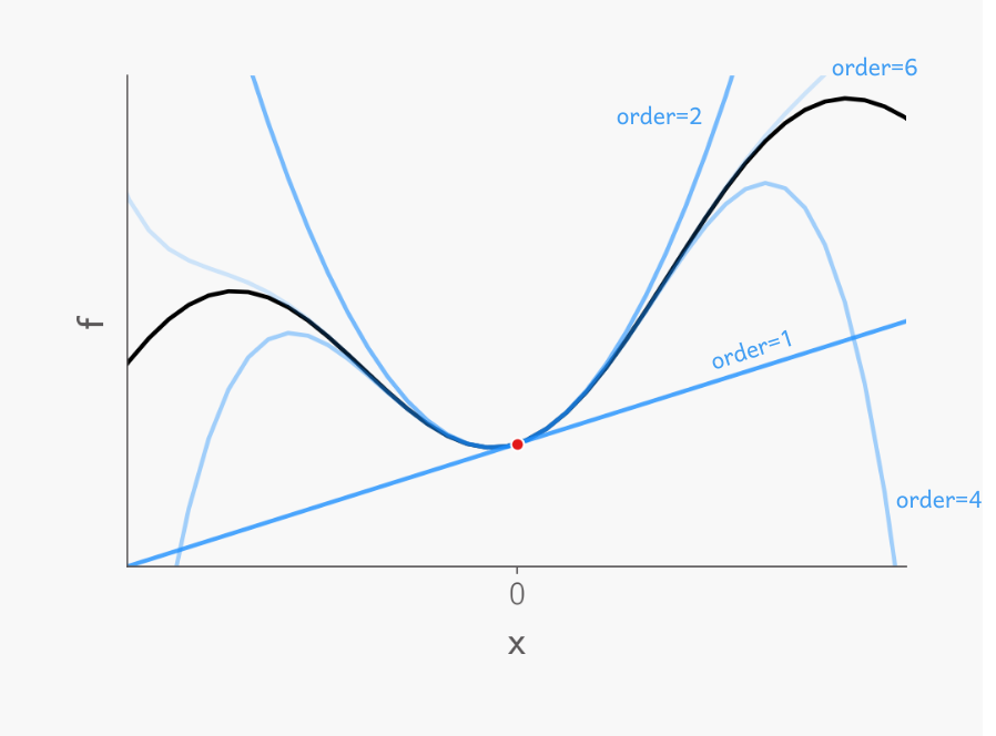
Newton’s method is rooted in the Taylor Series, a powerful mathematical tool that allows us to approximate complicated functions with a series of simpler terms. Mathematicians often develop such series to express intricate functions, where the first few terms dominate, and the remaining terms can often be safely ignored. By calculating these initial terms, we can efficiently estimate the behaviour of a function.

The Taylor Series expresses any function as a sum that looks like this:

In this equation, the exclamation mark represents a factorial: for example, 1! equals 1, 2! equals 2×1, and 3! equals 3×2×1, and so on. The dash symbol indicates a derivative, with a single dash representing the first derivative — the gradient of the function, or how rapidly the function’s value changes with respect to the input variable.

What this means in practical terms is that if you make a small change (??) to the input of a function, the resulting function value can be approximated by the right side of the equation. This includes the original function value at the unperturbed location, plus the gradient at that point multiplied by the small change, along with additional terms if needed.

Graphically, this can be visualised as follows: imagine a function shown as a black curve. Performing a Taylor Series expansion is like fitting a line to this curve. If we use only the first term, the approximation is a tangent line to the function, representing the gradient at that point. As we include more terms, the approximation becomes increasingly accurate, capturing more of the function’s true behaviour.

Newton’s Method in 2D

Newton’s method is highly versatile and can be applied to complicated functions, including those with multiple input variables in higher dimensions. However, to build a solid understanding of its inner workings, it’s helpful to start with a more familiar two-dimensional context.

In this section, we’ll explore the fundamentals of Newton’s method and visualise its application in two dimensions. By examining its derivation and visual behaviour in this simpler setting, we can more easily grasp the method’s principles before tackling more abstract, higher-dimensional scenarios.

Residual Form of Functions

To standardise the representation of both implicit and explicit, as well as linear and nonlinear functions, they are often expressed in the more generic residual form. Here is an example:

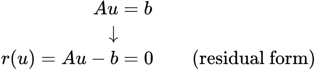
The term “residual form” comes from its use in numerical analysis, particularly in iterative methods. In this context, the right side of the equation represents the residual value. Initially, this value is large, indicating that the solution is not yet accurate. However, as iteration progresses, the residual ideally decreases towards zero, reflecting improved accuracy. Any remaining value at the end of the computation is referred to as the residual.

Derivation of Newton’s Method

Newton’s method utilises the Taylor Series to approximate a function in residual form, including up to the linear term. This approach is often referred to as a linear approximation. In this method, ? represents the initial guess, while ?? denotes the step size to the next guess. The goal is to find the value of ? that solves the equation such that the residual on the right side of the equation actually becomes zero.

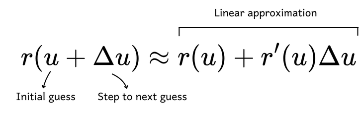
We assume that the step size (??) will drive us towards a solution where the residual is zero. By rearranging the equation, we can express ?? as:

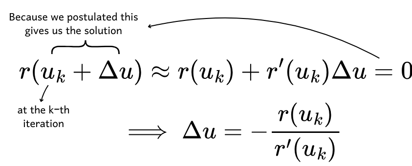
Since ?? represents the difference between the current estimate and the next estimate, we can write:

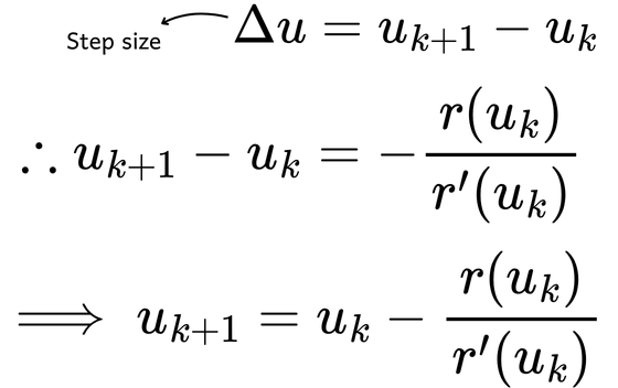
This formula provides the Newton update rule, which specifies that to obtain a new guess of ?, we subtract the function value divided by the gradient at the current step from the previous guess.

Newton’s Method in Action

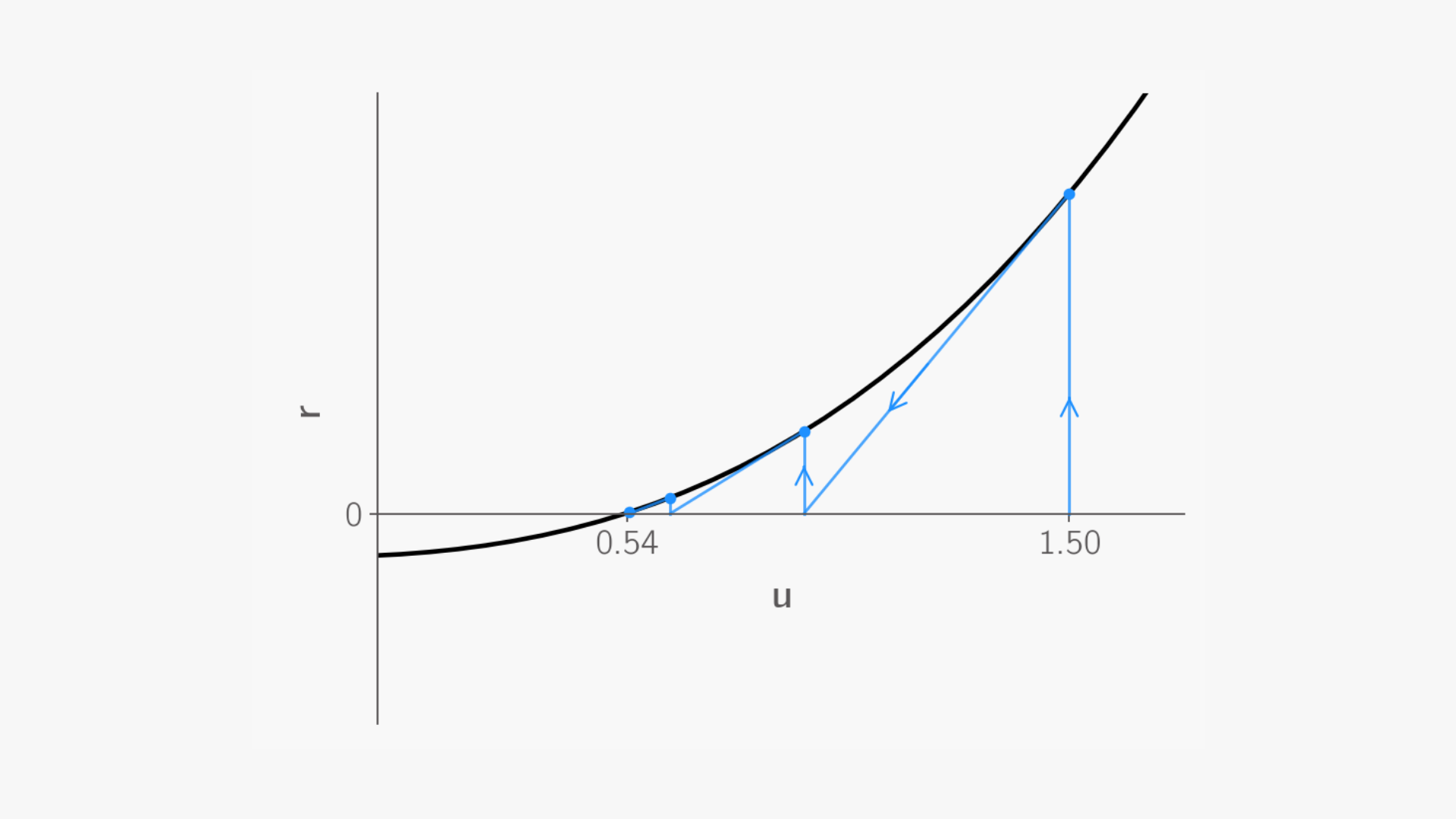
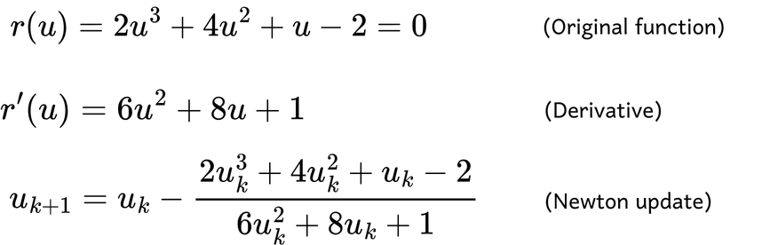
Consider the following function, with its derivative and Newton update given by:

Let’s start with an initial guess of ?=1.5. Graphically, this involves drawing a vertical line from the x-axis at ?=1.5 to its intersection with the function. At this intersection point, we approximate the function using a tangent line, as demonstrated with Taylor Series up to the linear term.

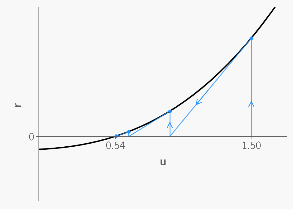
Following this tangent line towards the x-axis gives us our first update. Using this updated guess, we repeat the process: draw a vertical line from the x-axis to the new intersection with the function, fit a tangent line, and find where it intersects the x-axis to determine the next update.

After several iterations, this process converges to the root of the function, where the function intersects the x-axis, providing us with the solution.

Estimating Derivative

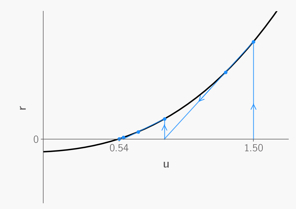
When the derivative of a function is difficult to compute or not directly available, we can estimate it using methods such as finite differences. The derivative is approximated with the following formula:

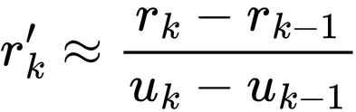
To estimate the derivative, we need two points near the point of interest. The derivative is approximated by the difference in the y-values divided by the difference in the x-values, which is essentially the gradient calculated as ??/??.

In two dimensions, this approach is known as the secant method. Instead of fitting a tangent line, the secant method fits a line between two points on the function, which extends to the x-axis to provide next update.

Extending Newton’s Method to Higher Dimensions

Newton’s method extends to higher dimensions in a manner similar to the two-dimensional case, though the equations now involve vectors and matrices, which can seem intimidating. However, grasping the fundamental concepts behind these terms is key to understanding the method.

In the following section, we’ll explore Taylor Series and Newton’s method in N dimensions, revealing that the core principles are fundamentally consistent with what we’ve seen in lower dimensions. Let’s dive into these higher-dimensional concepts and see how they align with the familiar principles of Newton’s method.

Revisiting Taylor Series and the Newton Update

The equation below represents Taylor Series in N dimensions. In this higher-dimensional context, we need to account for the direction of perturbation. Thus, for a small change in the input, originally denoted as ??, we now use ??. Here ? is the direction vector, and ? is a scalar indicating the magnitude of the perturbation in that direction.

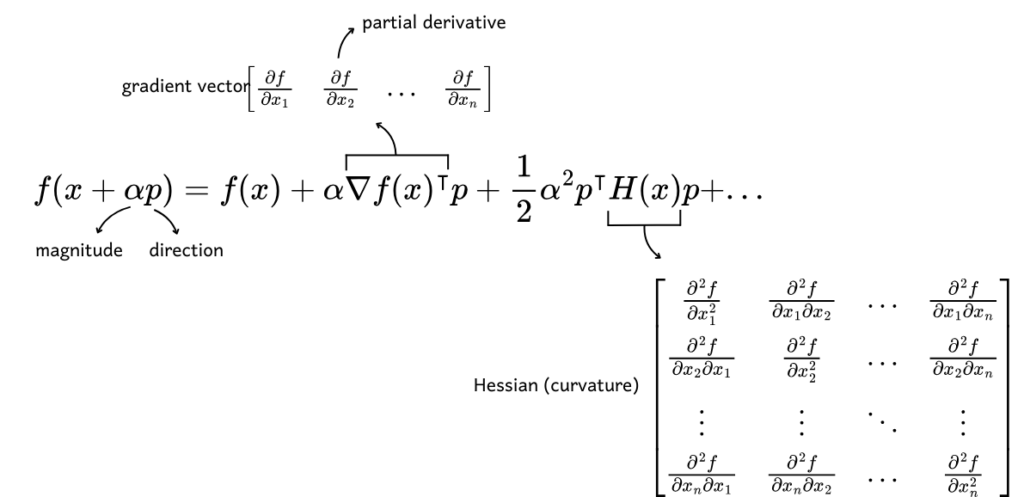
On the right side of the equation, instead of ?’(?)??, we have ???(?)??, where ??(?) is the gradient vector containing the partial derivatives of the function with respect to each input variable. The ? symbol denotes the transpose, allowing it to be multiplied with the ? vector correctly. For the quadratic form, we replace ?’’(?) with the Hessian matrix ?(?), which includes the second partial derivatives of the function with respect to combinations of input variables.

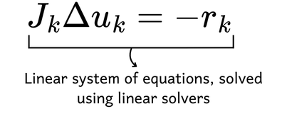
Using the N-dimensional Taylor Series, we can derive the Newton update as shown in the equation below. This method is particularly useful for solving nonlinear systems of equations, where we have multiple functions to solve simultaneously and aim to find a common value ? that satisfies all equations, representing their intersection point.

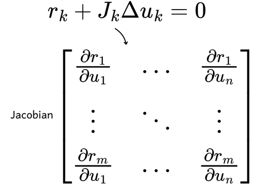
In this case, we use the Jacobian matrix ?, which replaces ?’(?) from the lower-dimensional case. The Jacobian matrix contains the partial derivatives of all functions in the system with respect to all variables. Substituting numerical values into this matrix equation reduces it to a linear system, which can be solved using standard linear solvers.

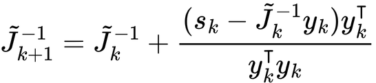
To estimate the Jacobian matrix, methods similar to the secant method can be employed. One such method is Broyden’s method, which provides an estimated Jacobian using the following equation:

Visualising Multidimensional Newton’s Method

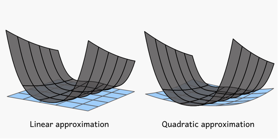
In three dimensions, approximating a function evolves from fitting a line to fitting a surface. A linear approximation in this case is represented by a plane, whereas incorporating higher-order terms approximates the function with a curved surface.

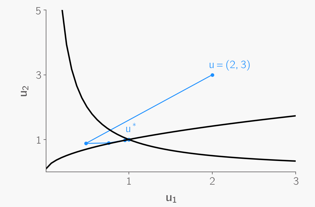
Newton’s method for solving nonlinear systems of equations can be illustrated as follows. Consider two nonlinear functions that intersect at ?? = ?? = 1, which represents the solution. Starting from an initial guess of ? = (2, 3), Newton’s method iteratively fits a surface to both functions, progressively refining the estimate until it converges to the intersection point.

Conclusions

Newton’s method is a powerful and ingenious technique for solving even the most complicated functions, known for its quadratic rate of convergence which makes it exceptionally efficient. It has many variations and applications across numerical analysis and optimization, and remains a favourite among practitioners.

In this article, we explored how Newton’s method operates and its connection to Taylor Series. We also generalised these concepts to higher dimensions and used visualisations to gain a more intuitive understanding of their inner workings. I hope you found this exploration both informative and engaging. If you have suggestions for other algorithms you’d like to see covered, please leave a comment below!

At OptimiSE Academy, we’re excited to announce our upcoming microcourse on Optimization Mathematics. This course aims to provide a comprehensive and intuitive foundation for anyone interested in design optimization. If you’re interested, sign up for the waitlist now using this link!